Introduction
In 2019 I set out to build an agent that could play Space Invaders. It was when I was first learning Machine Learning, and I never had the chance of completing the project. My free EC2 credits ran out, and I abandoned the project with an agent that could barely perform better than a random agent.
In 2024 I decided to resurrect the project. I had a job and I could easily afford to buy some EC2 credits to train the agent. However, it was impossible to get the project back and running: none of the libraries were pinned and some libraries were out of date and were no longer supported. In short, it was less effort to start the project from scratch.
This time I decided to use PyTorch instead of Keras, which my older version used. I went back to the papers and built the model from scratch based on the original 2013 paper Playing Atari with Deep Reinforcement Learning. By the time the model was good to be trained I got stalled again. The thought of setting up AWS for model training was more work than I wanted to take on in my free time. So the project was abandoned once more.
In October 2026 I had the bright idea of resurrecting my good ol’ gaming PC and turning it into a training machine: install Ubuntu Server and leave models running for days. After all, it’s got an OK GPU by modern standards (an RTX 2060) and should be able to tackle a good range of ML training problems.
With this new setup I was finally able to make my dreams come true, and train a reinforcement learning agent capable of deliberately playing Space Invaders!
Throughout this blog post I’ll walk through my implementation then and now, comparing the results and performance.
2019 and 2026, side by side, at double speed. The 2019 agent’s game ends on 235 points while the 2026 agent scores 2,050.
Domain Background
Reinforcement learning works by maximising a value function, where the agent chooses the actions that maximise the expected reward. Advances in deep learning, especially in computer vision, have let reinforcement learning algorithms use neural networks as function approximators. These work far better than older techniques when the state space is continuous, such as raw screen pixels.
Atari games used to be the benchmark for reinforcement learning when the Deep Q-Network (DQN) algorithm was introduced (Mnih et al., 2013). In 2015 the same team showed, in a paper in the journal Nature, that a DQN could reach human-level scores across dozens of Atari games, all learnt from pixels with the same network and settings (Mnih et al., 2015).
The motivation for this project is to recreate that algorithm for Space Invaders and see how close I can get to a human player.
Problem Statement
The problem can be framed as a Markov Decision Process (Sutton and Barto, 2018), where the agent is the learner making the decisions and the environment is the Atari emulator. At each time step t, the agent selects an action from a discrete set of actions A = {1, …, K}. One time step later, as a consequence of that action, the agent receives a new state S(t+1) from the emulator as an image, and a reward R(t+1) based on how the score changed. Repeating this produces a trajectory:
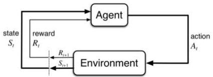
The Markov Decision Process: the agent acts, and the environment answers with a new state and a reward.
The goal of the agent is to select the actions that maximise the expected return. Future rewards are discounted by a factor γ per time step, so the return from time t is:
$$ G_t = \sum_{k=0}^{\infty} \gamma^k R_{t+k+1} $$In Space Invaders the agent controls a cannon at the bottom of the screen with 6 actions: do nothing, fire, move right, move left, and move right or left while firing. Points come from shooting invaders, and the game ends when the agent has lost all 3 lives.
Datasets and Inputs
There is no fixed dataset: the agent generates its own data by playing. Rather than building my own Space Invaders clone, I use the ALE/SpaceInvaders-v5 environment from Gymnasium, the maintained successor to OpenAI Gym, which runs the original Atari 2600 game through the Arcade Learning Environment. In 2019 I used OpenAI Gym itself.
The agent only receives raw pixels, the same as a human sees on the screen, and it learns to play from scratch based on its own experience and rewards. Each input goes through these steps:
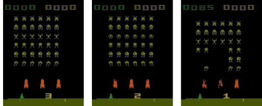
Raw input frames, showing where the agent starts with 3, 2 and 1 lives left.
- Greyscale and resize. The 210 × 160 colour frame becomes an 84 × 84 greyscale image.
- Frame skipping. Each chosen action is repeated for 3 frames, so the agent decides 20 times a second rather than 60.
- Frame stacking. The last M = 4 frames are stacked, so the agent can see movement, such as which way a bullet is travelling. The final state is 4 × 84 × 84.
- Scaling. Pixel values are divided by 255 inside the network, so inputs sit between 0 and 1.
- Reward clipping. For training, each reward is clipped to between −1 and +1, so every invader counts the same. The real, unclipped game score is recorded separately and is what I report.
In my original implementation back in 2019 I tried to write my own preprocessing pipeline with OpenCV. It was slow enough to crash my computer early in training.
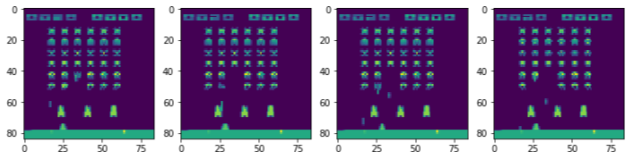
A stack of 4 preprocessed frames, as one input to the network. This is from my 2019 version, which cropped out the score and the ground and showed the frames in false colour. The current version keeps the full frame at 84 × 84.
I switched to the environment’s own wrappers, which are much more efficient and convenient.
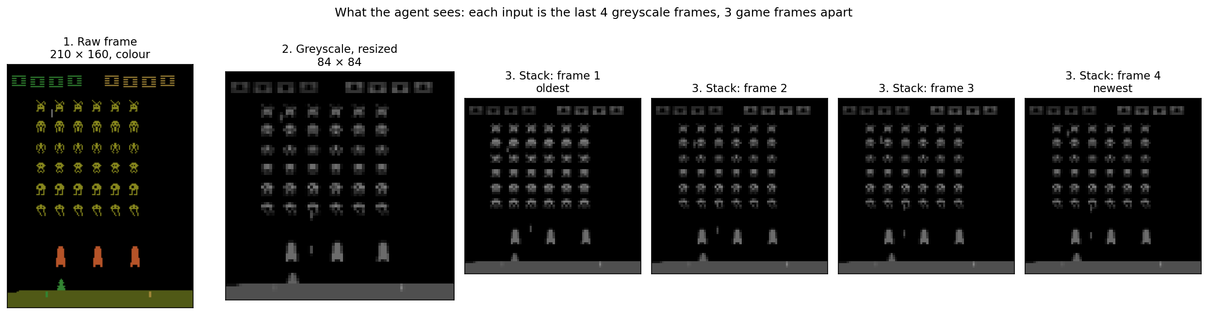
The current pipeline, from the 2026 code: the raw 210 × 160 colour frame, the same frame in greyscale at 84 × 84, and the stack of the last 4 frames that the network actually receives. Look closely at the bullet between the cannon and the shields: it moves up between frames, which is how the agent can tell which way things are travelling.
Solution Statement
The solution is a Deep Q-Network: a convolutional neural network that looks at the last 4 frames and estimates how much future score each of the 6 actions is worth.
The agent chooses actions based on a policy π, a mapping from a state s to an action a. The action-value function gives the expected return if the agent starts in state s, takes action a, and follows the policy afterwards. Bellman’s optimality equation expresses the value of any state in terms of the states that could follow it:
$$ Q^*(s, a) = \mathbb{E}\left[ R_{t+1} + \gamma \max_{a'} Q^*(S_{t+1}, a') \mid S_t = s, A_t = a \right] $$In temporal-difference learning this becomes an update rule applied at every step:
$$ Q(S_t, A_t) \leftarrow Q(S_t, A_t) + \alpha \left( R_{t+1} + \gamma \max_a Q(S_{t+1}, a) - Q(S_t, A_t) \right) $$In traditional Q learning, there is a Q table which holds all the possible next state values for each possible action. For a non-discrete environment like Space Invaders, a table can’t hold a value for every possible screen, it’s simply not feasible. Instead, we use a convolutional network with weights w that approximates Q instead. The estimated return at the next step becomes the target, computed with a separate copy of the weights, w⁻, that stays fixed for a while (fixed Q-targets):
$$ y = R_{t+1} + \gamma \max_a Q(S_{t+1}, a; w^-) \qquad \Delta w = \alpha \left( y - Q(S_t, A_t; w) \right) \nabla_w Q(S_t, A_t; w) $$In practice the network is trained to minimise the Huber loss between y and its prediction. The Huber loss is squared for small errors and linear for large ones, so one surprising transition can’t produce a huge gradient. In 2019 I used a plain squared error, which is much less forgiving.
To balance exploration and exploitation, the agent follows an ε-greedy policy. With probability ε it picks a random action, and otherwise it picks the action with the highest Q-value. ε starts at 1 (pure exploration) and is multiplied by 0.9985 after every game until it reaches a floor of 0.01, which run 2 reached after about 3,000 games.
The network: starting small, then going bigger
My original 2019 implementation used the larger network as presented in the 2015 Nature paper, with a dueling head on top. But because it performed so poorly, when I rebuilt the project in 2024 I decided to take a step back, and use the smaller network originally presented in the 2013 paper. I also thought there was a chance I could try to train this on my MacBook. Spoiler alert, it still wasn’t feasible.
That small network did learn, but it hit a ceiling. Its average peaked at 503 points and then slowly fell as training continued. For the next training run, I switched to the Nature-sized network as well as modifying some of the training settings (see the change log below).
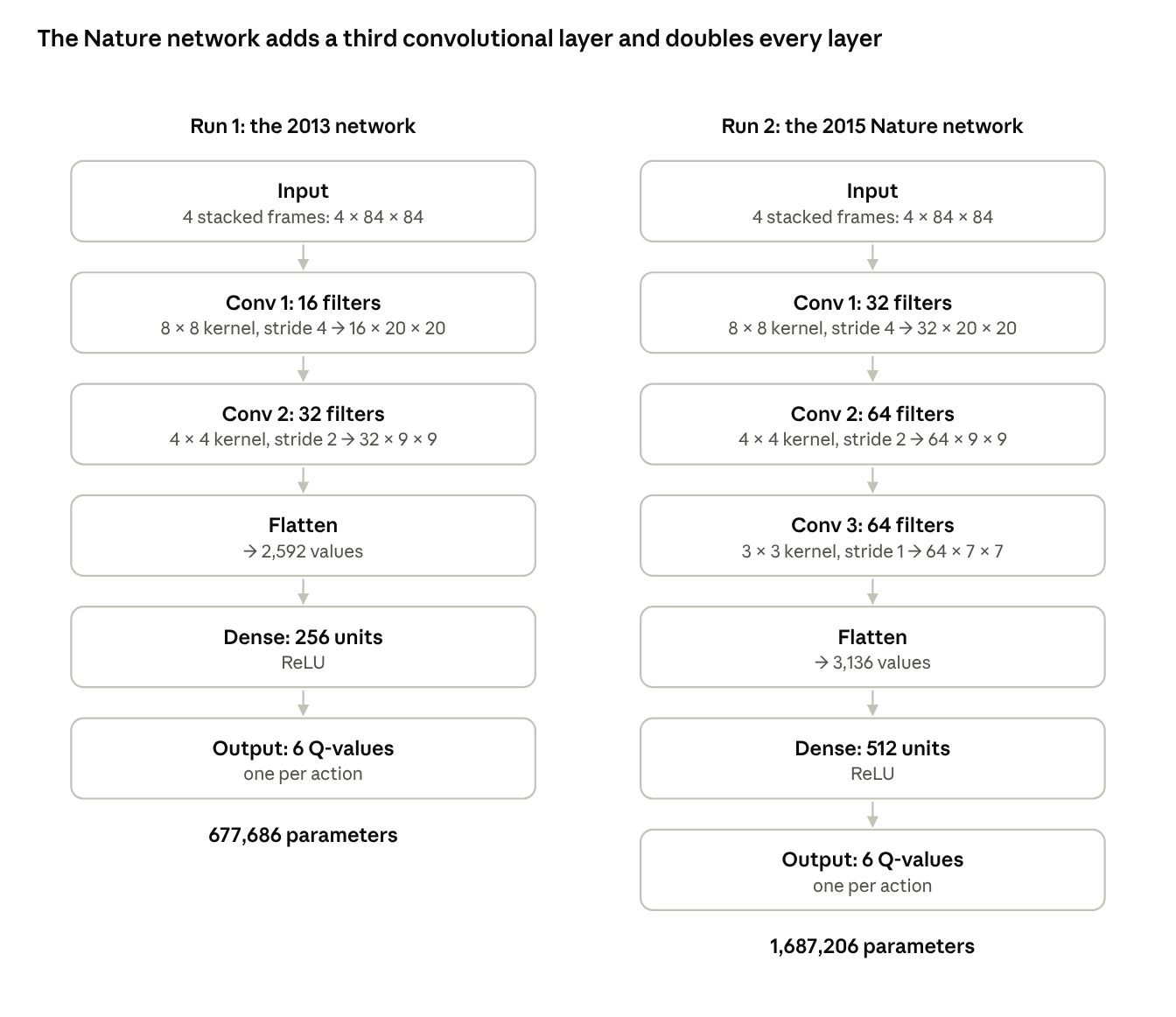
From src/q_function.py, before and after the November 2026 change.
Both networks take the same 4 × 84 × 84 input and output one Q-value per action. The Nature network adds a third convolutional layer and doubles the width of every other layer, which takes the parameter count from 677,686 to 1,687,206.
Benchmark Model
The main benchmark is still a professional human games tester, who averaged 1,652 points in the 2015 Nature paper. The idea behind reinforcement learning is for computers to learn by interacting with an environment, much as humans do, so a human player is the natural benchmark.
| Benchmark | Average score | Where it comes from |
|---|---|---|
| Random agent | 148 | Nature paper, 2015 |
| DQN, small network | 581 | Mnih et al., 2013 |
| Professional human tester | 1,652 | Nature paper, 2015 |
| DQN, Nature network | 1,976 | Nature paper, 2015 |
A random agent scoring 210 points.
Evaluation Metrics
The main metric is the agent’s real game score, averaged over the last 100 games. In supervised learning you can split a dataset into training, validation and test sets. In reinforcement learning, evaluating the model isn’t as straightforward, so I watch how the agent performs over time. Every game is logged with these numbers:
- Game score. The actual, unclipped Space Invaders score, the same number a human player would see on screen.
- 100-game moving average. A single game is very noisy: the same agent can score 400 one game and 1,500 the next. The model with the highest 100-game average is saved separately as
best.pt, so a later decline in training can’t lose it. - Loss. The Huber loss between the network’s predictions and its targets. It doesn’t fall steadily as it would in supervised learning. What matters is that it settles into a stable band rather than climbing without limit.
- Epsilon and training time. These show how much the agent is still exploring and how long each result took.
The scores I report are measured during training, so the agent still takes a random action some of the time: 1% in run 2, and 10% in run 1.
For the final model, I also ran an evaluation over 100 games with no random moves, reported under Results.
Project Design and Results
The design is the same DQN I proposed in 2019, with some improvements made along the way.
Design
Training a neural network on its own experience is unstable: consecutive frames are highly correlated, and the targets move as the network learns, so the weights can diverge. Two techniques from the DQN papers deal with this:
- Experience replay. Each (state, action, reward, next state, done) tuple is saved in a replay memory of 100,000 transitions. Training batches of 32 are sampled at random from it, which breaks up correlated sequences and lets the agent recall unusual situations more than once. Frames are stored as 8-bit integers, so the full memory fits in about 6 GB of RAM.
- Fixed Q-targets. The targets are computed with a copy of the network, w⁻, which is only updated to match the live weights w every 10,000 steps. This decouples the target from the weights being updated.
The algorithm interleaves two processes. One plays the game and stores each transition in the replay memory. The other, every 4 steps, samples a batch and takes one gradient-descent step on it. In run 2, learning only starts once the memory holds 50,000 transitions, so the first updates aren’t fitted to a handful of games. Run 1 started after just 500.
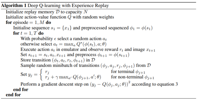
The DQN algorithm from Mnih et al. (2013), as I included it in my 2019 proposal. The current version follows it, with the changes listed below.
Training specs
Hardware
| 2019 | 2026 (both runs) | |
|---|---|---|
| Machine | AWS EC2 p2.xlarge | Home PC |
| OS | Ubuntu Server | Ubuntu Server 26.04 LTS |
| GPU | NVIDIA Tesla K80 (one GPU, 12 GB) | NVIDIA GeForce RTX 2060 (6 GB) |
| CPU | 4 virtual CPUs | AMD Ryzen 5 3600 (6 cores, 12 threads) |
| RAM | 61 GB | 16 GB |
| Software | Python 3, TensorFlow with Keras, OpenAI Gym (SpaceInvaders-v0); versions not recorded | Python 3.10, PyTorch 2.14 with CUDA 13, Gymnasium 1.4, Arcade Learning Environment 0.12 |
Training
| 2019 Run | Run 1: small network | Run 2: Nature network | |
|---|---|---|---|
| Training time | 17 h 56 min | 31 h 37 min | |
| Time to best model | 5 h 4 min | 27 h 10 min | |
| Training steps | about 29 million | 28,218,535 | 44,845,815 |
| Games played | 40,000 | 29,288 | 28,667 |
| Speed | 436 steps a second | 394 steps a second | |
| Gameplay seen | about 86 million frames, roughly 17 days of real life play | about 85 million frames, roughly 16 days of real life play | about 135 million frames, roughly 26 days of real life play |
Training ran on my RTX 2060 with a single script I could leave running in the background. Before that, I briefly tried training on Google Colab, which kept disconnecting every two hours.
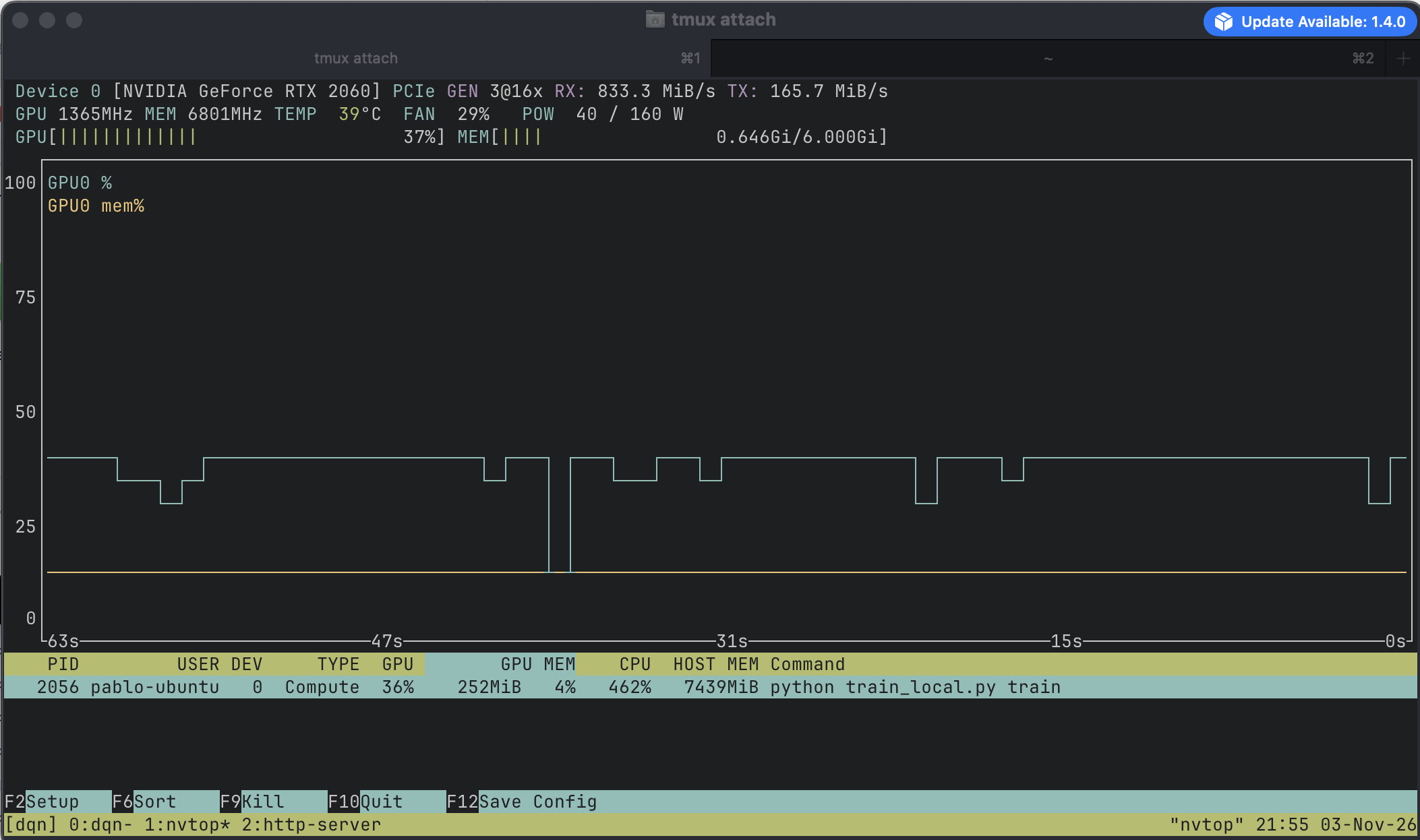
Run 2 training, watched with nvtop inside tmux. The GPU sits at about 37% utilisation, draws 40 of its 160 W, and runs at 39°C. The training script uses only 252 MiB of the GPU’s 6 GB, but about 4.6 CPU cores and 7.4 GB of RAM, most of it the replay memory. The work is mostly on the CPU side, running the game.
Log History of changes made
| Date | Change | Why |
|---|---|---|
| Nov 2026 | Switched to the Nature-sized network | The small network hit a ceiling (see Results) |
| Nov 2026 | Adam optimiser (learning rate 0.0001) instead of RMSprop | RMSprop with PyTorch’s default settings made jumpy updates, the likely cause of the decline in run 1 |
| Nov 2026 | Losing a life counts as the end of a sequence in the replay memory | The agent learns that dying cuts off future points, without restarting the game |
| Nov 2026 | Exploration floor lowered from 10% to 1%; learning waits for 50,000 transitions | Fewer random moves late in training; a less biased start |
| Oct 2026 | Discount factor raised from 0.9 to 0.99; faster ε decay | 0.9 only looks about 10 steps ahead, too short for a bullet to reach an invader |
| Oct 2026 | Replay memory raised from 10,000 to 100,000, stored as 8-bit | More varied memories without running out of RAM |
| Oct 2026 | Squared error replaced with Huber loss; learn every 4 steps | More stable updates, as in the papers. My 2019 version only learnt once per game |
| Oct 2026 | Pixel values scaled to between 0 and 1 | The network was being fed raw 0 to 255 values |
| Mar 2024 | Rewrote the project in PyTorch with the 2013 small network | A clean restart, starting small to train faster |
| Mar 2019 | Built the first model version |
Results
Each attempt beat the last: my 2019 agent averaged about 190 points, run 1 reached 503.5, and run 2 reached 1,175.6.
| Attempt | Network | Training steps | Best average score |
|---|---|---|---|
| 2019, Keras | Nature-sized, with dueling head | about 29 million (estimated) | about 190 |
| 2026, run 1 | 2013 small network | 28.2 million | 503.5 |
| 2026, run 2 | Nature-sized network | 44.8 million | 1,175.6 |
The 2019 code didn’t log steps, so its figure is an estimate: 40,000 games at about 720 steps each, the length of a near-random game in my 2026 runs. It’s counted in 2026-sized steps of 3 frames. The 2019 agent skipped about 12 frames per step, so it actually made closer to 7 million decisions.
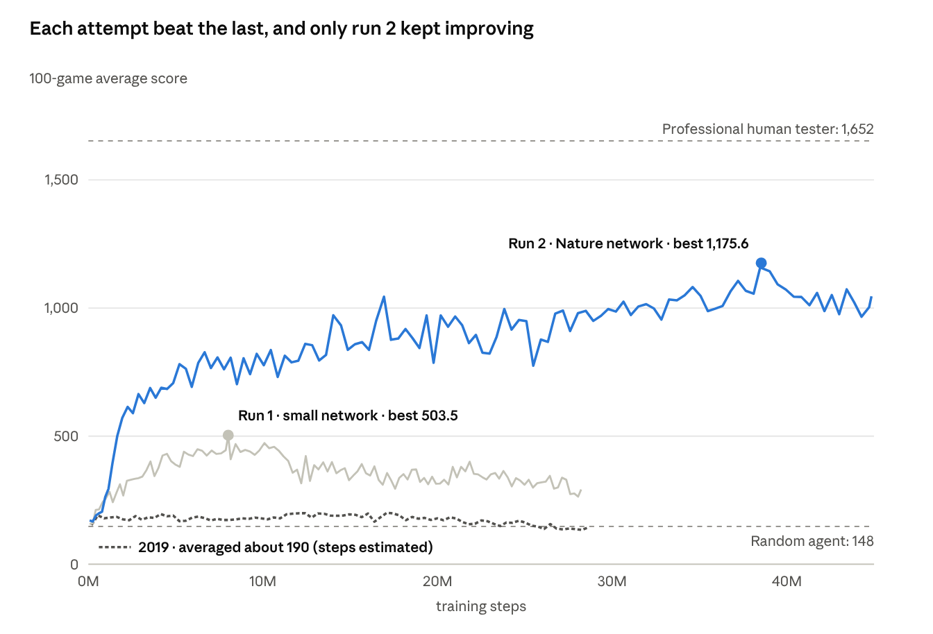
From progress.csv of both 2026 runs, 100-game average every 250 games. The 2019 line is traced from my 2019 report.
- 2019 (Keras): learnt a little, then went backwards. Its average rose for roughly the first half of training and then fell. Evaluated over 500 games, it averaged 190, barely above a random agent. Looking back at the code, the main reason is clear: it only learnt once per game, fitting 64 samples one at a time after each game ended. That’s about 2.6 million samples learnt from in total, against about 358 million for run 2.
- Run 1 (small network): learnt quickly, then stalled. Its best 100-game average was 503.5, after 8.0 million steps (5 hours). It then drifted down to 292 by the end, even though the loss stayed stable. Best single game: 1,695.
- Run 2 (Nature network): passed run 1’s best after only 1.6 million steps, about an hour in, and kept improving slowly for the next 27 hours. Its best 100-game average was 1,175.6, after 38.5 million steps. After that it levelled off rather than collapsing, and its last 100 games averaged 1,045.7. Best single game: 2,830.
Watching them play
Every attempt, playing at the same time. When a game ends, its panel goes dark and shows the final score: the random agent goes out after 13 seconds with 210 points, the 2019 agent after 43 seconds with 235, and run 1 after 73 seconds with 590. The final agent is still playing when the clip ends at 80 seconds.
The two 2026 agents on their own, each playing a full game:
Run 1’s best model playing one game: it lasts 73 seconds and scores 590 points.
Run 2’s best model, the final agent: scores 2,050 points over two and a half minutes.
How good is the final agent?
Playing with no random moves, the best model averaged 1,111.8 points over 100 games, with a best game of 2,375 and a worst of 410. That’s nearly double the 2013 DQN (581), but still below the professional tester (1,652) and the Nature DQN (1,976). Its best games beat both of those averages.
What it learnt
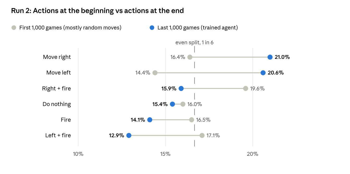
Action counts from run 2’s train_log.txt, first and last 1,000 of 28,667 games.
Early in training, while the agent is mostly exploring at random, each of the 6 actions gets close to an even share. By the end it has learnt to move far more than it fires: plain left and right moves rise from about 15% each to about 21%, and the fire actions drop from about 53% of moves to 43%. It spends more of its time dodging and lining up shots, rather than firing constantly.
Improvements
The two improvements I promised in 2019, prioritised experience replay and dueling networks, are not in the current version, and I’m leaving them as future work. This project’s comparison is run 1 against run 2. Run 2 changed several things at once (the network size, the optimiser, the life-loss signal and the exploration settings), so its gain over run 1 comes from all of them together rather than from any single change. I’m not planning further runs to test each change on its own.
If I come back to it, these are the changes I’d try, most promising first:
- N-step returns. Use the sum of the next 3 rewards as the target instead of just one. When the agent fires, the bullet takes dozens of steps to reach an invader, so the credit for a good shot should flow back faster. This is the cheapest change and, according to the Rainbow paper (Hessel et al., 2018), one of the two that matter most.
- Double DQN. Let the live network choose the next action and the target network score it. This reduces the overestimation of Q-values, a common cause of scores declining late in training.
- Prioritised experience replay. Replay the transitions the network got most wrong more often (Schaul et al., 2015). This is the one I couldn’t get working in 2019.
- Dueling network. Split the last layer into a state value and an advantage for each action, as I did in 2019 (Wang et al., 2015).
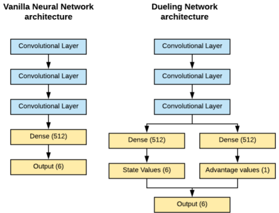
From my 2019 report: the plain network next to the dueling network I used then. The dueling version splits after the convolutional layers into one stream for the state’s value and one for each action’s advantage, then combines them into the 6 Q-values.
Closing thoughts
The goal I set in 2019 was to make an agent capable of playing Space Invaders. What I’ve got now is an agent that clearly understands the game, and is capable of beating the first level almost every time. In some games it scores higher than the human tester baseline at 1,652 points.
It’s very unlikely that I’ll revisit this project again, but it has been deeply satisfying to see this project realised. Reinforcement learning has a special place in my heart, and it makes me happy to finally have it successfully implemented.
This project has also opened my eyes to the incredible opportunities of AI assisted programming for ML work. While I built all of the model architecture myself, I used AI as an advisor for potential issues in the code or for advice on which parameters to pick. It has also been immensely useful to hand over all of the checkpointing, charts, logging and all other important yet tiresome and slow work to the agent, so I could simply focus on running the script and observing the results.
Next, I’ll probably spend more time with language models. Now that I have my GPU home lab I can start training my own language models, which I’m very excited about.
Until next time!
Appendix: detailed training charts
The full charts behind the summary in Results, including the training loss, which the summary chart leaves out.
2019 attempt
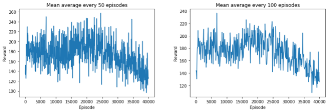
2019: average reward per 50 and per 100 episodes over 40,000 episodes of training.
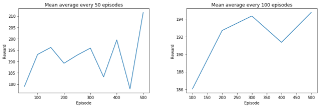
2019: evaluating the trained agent over 500 games. The average settled at about 190.
At the time, I suggested that perhaps there were signs of deliberate play. In this sequence, the agent moves under cover to dodge an incoming bullet, however, this was likely a fluke, considering the agent barely got better than the random agent.
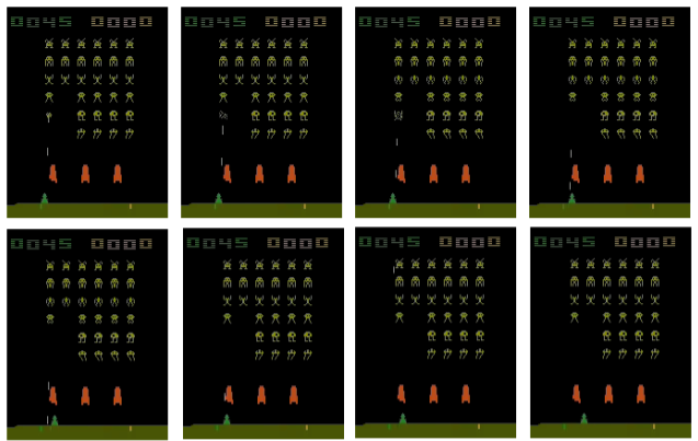
2019: eight consecutive frames, left to right, of the agent "taking cover to dodge a bullet".
Run 1: small network
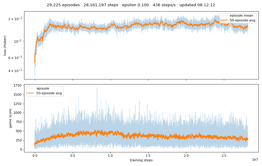
Run 1’s training chart: 29,288 games and 28.2 million steps over 17 h 56 min. The loss stays stable, while the score peaks at about 8 million steps and then declines.
Run 2: Nature network
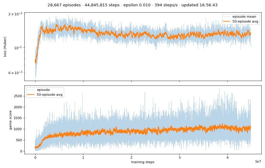
Run 2’s training chart: 28,667 games and 44.8 million steps over 31 h 37 min. The loss settles early and stays stable, and the score keeps rising slowly until about 38 million steps.
References
- Hessel, M., Modayil, J., van Hasselt, H., Schaul, T., Ostrovski, G., Dabney, W., Horgan, D., Piot, B., Azar, M. and Silver, D. (2018). Rainbow: Combining Improvements in Deep Reinforcement Learning. AAAI.
- Mnih, V., Kavukcuoglu, K., Silver, D., Graves, A., Antonoglou, I., Wierstra, D. and Riedmiller, M. (2013). Playing Atari with Deep Reinforcement Learning. arXiv.
- Mnih, V., Kavukcuoglu, K., Silver, D., Rusu, A. A., Veness, J., Bellemare, M. G., Graves, A., Riedmiller, M., Fidjeland, A. K., Ostrovski, G., Petersen, S., Beattie, C., Sadik, A., Antonoglou, I., King, H., Kumaran, D., Wierstra, D., Legg, S. and Hassabis, D. (2015). Human-level control through deep reinforcement learning. Nature, 518.
- Schaul, T., Quan, J., Antonoglou, I. and Silver, D. (2015). Prioritized Experience Replay. arXiv.
- Sutton, R. and Barto, A. (2018). Reinforcement Learning: An Introduction. 2nd ed. Cambridge, Massachusetts: The MIT Press.
- Wang, Z., Schaul, T., Hessel, M., van Hasselt, H., Lanctot, M. and de Freitas, N. (2015). Dueling Network Architectures for Deep Reinforcement Learning. arXiv.
Project code: original 2019 project · current version.