Without non-linear functions, neural networks can’t learn complex patterns.

This is a basic fact about what makes neural networks useful. If we don’t add non-linear functions such as ReLU to the hidden layer outputs outputs, a model will just end up as a simple linear model, no matter how complex the model might seem at a first glance.

The purpose of this blog is to clearly prove this. But before I can get to the proof, I’ll set the scene first.

A single neuron model

Throughout this blog I’ll be using a specific nomenclature, so I wanted to define the basics here and build up from there.

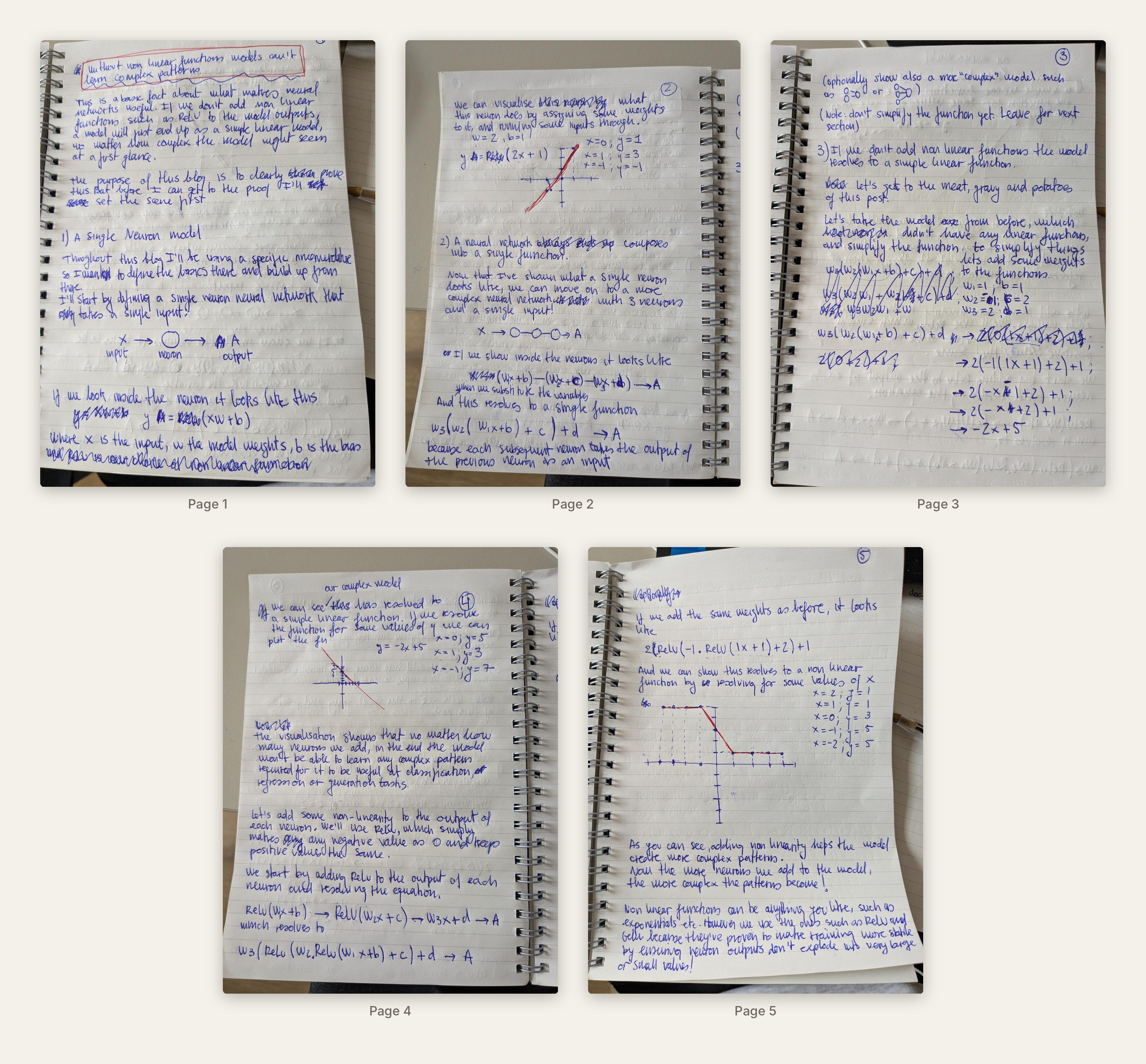
I’ll start by defining a single neuron neural network that takes a single input:

If we look inside the neuron, it looks like this:

$$y = xw + b$$

where \(x\) is the input, \(w\) the model weights, \(b\) is the bias and \(y\) is the output.

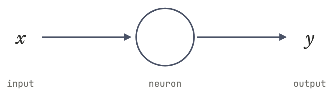
We can visualise what this neuron does by assigning some random weights to it

$$w = 2,\quad b = 1$$$$y = 2x + 1$$

and running a few values of \(x\) through it. Plotting the \(y\) we get for each input gives us:

What we get is a straight line. In plain terms, this model can only predict patterns that follow a straight line: as \(x\) goes up, \(y\) always goes up (or down) by the same amount. Changing the weights only tilts or shifts the line; it never bends it.

A neural network composes into a single function

Now that I’ve shown what a single neuron looks like, we can move on to a more complex neural network with 3 neurons and a single input!

If we show inside the neurons, it looks like

$$(w_1x + b) \rightarrow (w_2h_1 + c) \rightarrow (w_3h_2 + d) \rightarrow y$$

The first neuron takes \(x\) as the input. Subsequent neurons take as input the output from the previous neuron (\(h_1\) and \(h_2\)). When we substitute each neuron’s output into the next one, it resolves to a single function

$$w_3\big(w_2(w_1x + b) + c\big) + d \rightarrow y$$

If we don’t add non-linear functions, the model resolves to a simple linear function

Let’s get to the meat, gravy and potatoes of this post. Let’s take the function from before

$$y = w_3\big(w_2(w_1x + b) + c\big) + d$$

and simplify it. To better illustrate this, I’ll substitute the weights and biases with some random values like a real model starts with.

$$\begin{aligned} w_1 &= 1, & b &= 1 \\ w_2 &= -1, & c &= 2 \\ w_3 &= 2, & d &= 1 \end{aligned}$$$$y = 2\big(-1\,(1x + 1) + 2\big) + 1$$

If we resolve, we end up with

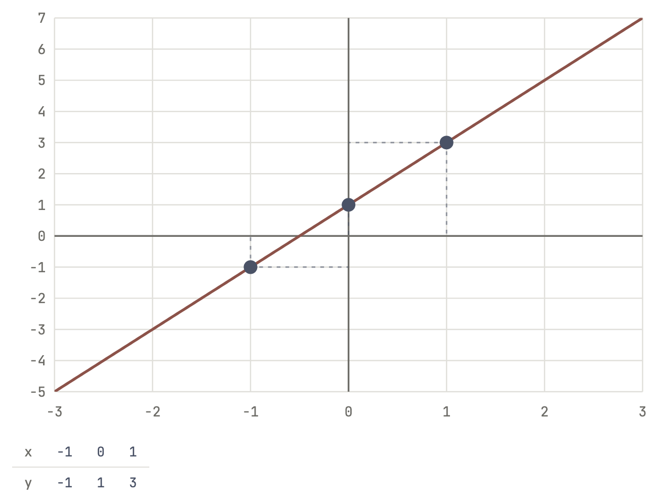
$$ \begin{aligned} y &= 2\big(-x - 1 + 2\big) + 1 \\[6pt] &= 2(-x + 1) + 1 \\[6pt] &= -2x + 2 + 1 \\[6pt] &= -2x + 3 \end{aligned} $$

As we can see, our complex model has resolved to a simple linear function. If we resolve the function for some values of \(x\), we can plot the function.

$$y = -2x + 3$$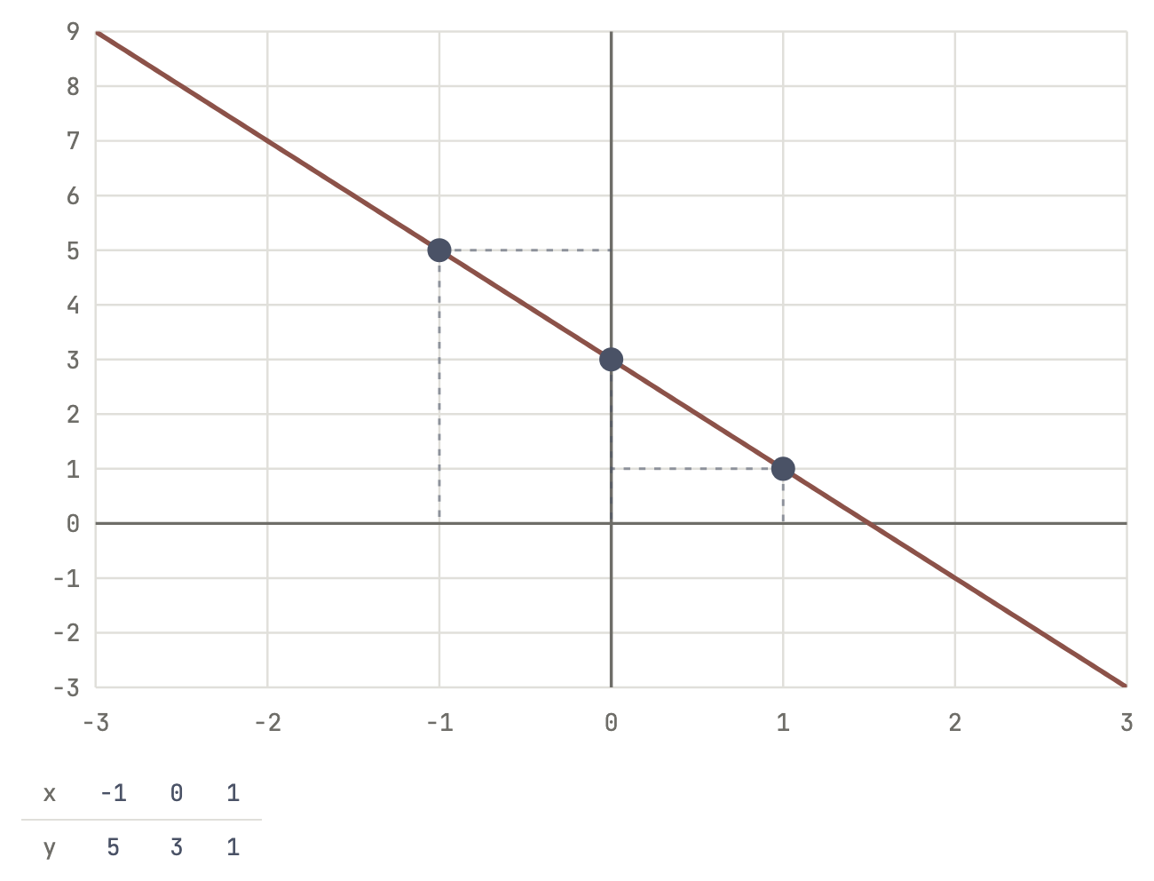

We used three neurons in a row here, but the same is true for bigger models where every neuron connects to every neuron in the next layer: all the multiplying and adding still collapses into one linear function.

No matter how many neurons or dimensions we add, without non-linearity the model won’t be able to learn any complex pattern required for it to be useful at classification, regression or generation tasks.

Adding non-linearity

Let’s add some non-linearity to the output of each neuron. We’ll use ReLU, which simply makes any negative value 0 and keeps positive values the same.

We start by adding ReLU to the output of each neuron and resolving the equation.

$$\mathrm{ReLU}(w_1x + b) \rightarrow \mathrm{ReLU}(w_2h_1 + c) \rightarrow w_3h_2 + d \rightarrow y$$

which resolves to

$$w_3\,\mathrm{ReLU}\big(w_2 \cdot \mathrm{ReLU}(w_1x + b) + c\big) + d \rightarrow y$$

If we add the same weights as before, it looks like

$$2\,\mathrm{ReLU}\big(-1 \cdot \mathrm{ReLU}(1x + 1) + 2\big) + 1$$

Unlike before, we can’t multiply the brackets out, because ReLU sits in the way. So the function can no longer collapse into a single straight line.

And we can show this resolves to a non-linear function by resolving for some values of \(x\).

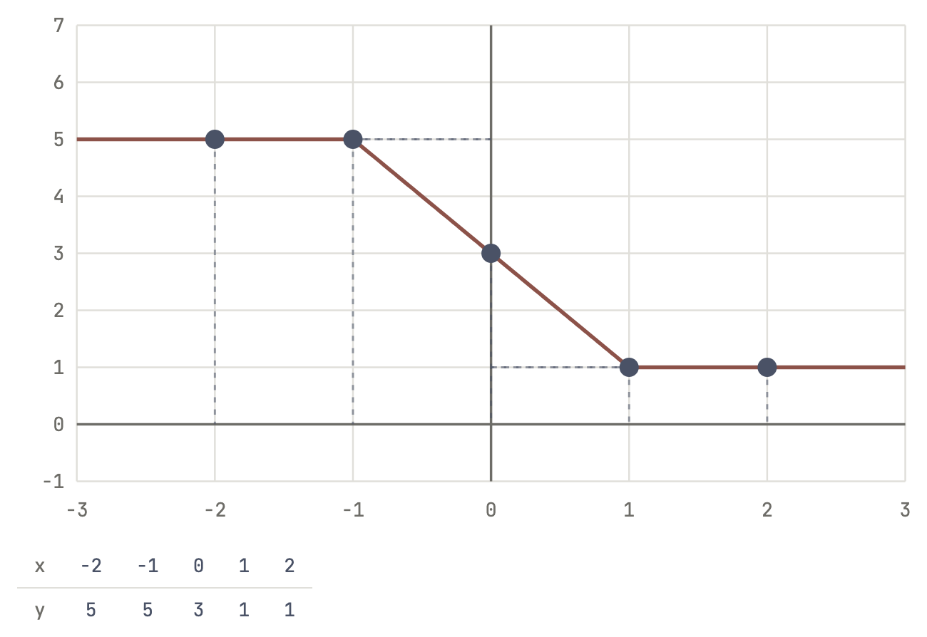
For \(x \ge 1\) the second neuron’s sum goes negative, so ReLU clips it to 0 and \(y\) stays at 1. For \(x \le -1\) the first neuron is clipped instead, so \(y\) stays at 5. In between, it’s the same line as before.

As you can see, adding non-linearity helps the model create more complex patterns.

Now the more neurons we add to the model, the more complex the patterns become, because each extra ReLU neuron can add another bend!

You can try doing this yourself by hand with different model shapes and sizes. Keep in mind that adding more than a single input will increase the dimensional space, making it tricky to visualise the results!

Non-linear functions can be anything you like, such as exponentials etc. However, we use ones such as ReLU and GELU because they’re cheap to compute and don’t squash gradients the way older functions like sigmoid do, which makes deep models much easier to train!

Appendix

Pen and paper drafts